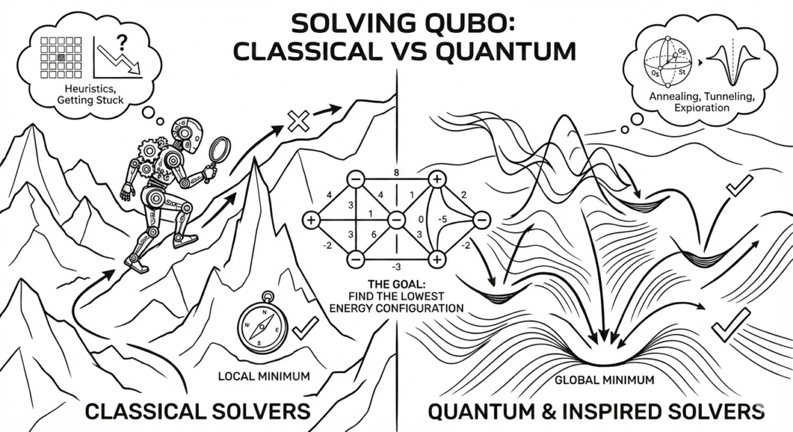
(Classical vs Quantum)
Goal of this chapter
By the end of this chapter, you will:
- Understand how QUBO problems are actually solved
- Connect the graph view (Chapter 4) to real solvers
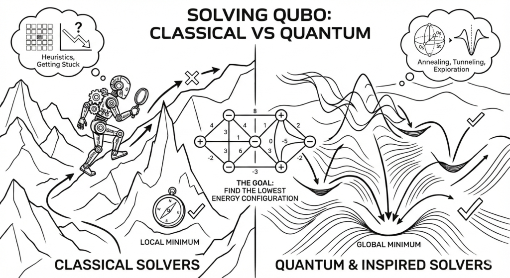
- See how annealing explores the energy landscape
- Understand why solvers get stuck in local minima
- Know clearly when you do not need a quantum computer
First Reality Check: QUBO Is Already the Hard Part
Once you have a QUBO: Your problem is finished conceptually.
All solvers (classical or quantum) are doing the same thing: Searching for the lowest-energy configuration of the graph.
From Chapter 4:
- Nodes want to turn ON
- Edges add cost when bad combinations happen
Solving QUBO means: Find a set of ON/OFF nodes that creates the deepest valley.
How Solvers See Your Problem (Graph View)
From a solver’s perspective:
- Node weights → hills or slopes
- Edges → cliffs or walls
The solver explores the graph by:
- Turning nodes ON or OFF
- Checking how energy changes
- Moving toward lower energy states
This is true for all solvers.
Two Big Families of Solvers
There are only two categories:
- Classical solvers (run on normal computers)
- Quantum / quantum-inspired solvers
They differ in how they explore the graph, not what they solve.
1. Classical Solvers (Used Most of the Time)
Brute Force (Learning Only)
- Try every possible combination
- Guaranteed correct answer
- Only works for very small problems
Graph intuition:
- Check every valley
- Pick the deepest one
Good for:
- Education
- Debugging
- Very small QUBOs
Local Search & Heuristics (Real World)
Most real QUBOs are solved using heuristics like:
- Simulated Annealing (SA)
- Hill Climbing
- Tabu Search
- Genetic Algorithms
These solvers:
- Start somewhere on the graph
- Flip a few nodes
- Move downhill if energy improves
Problem:
They can get stuck in local minima.
Why Local Minima Happen
From Chapter 4’s landscape view:
- A local minimum = small valley
- Global minimum = deepest valley
A solver may reach a valley where:
- All nearby moves go uphill
- But a deeper valley exists elsewhere
This is not a bug. It’s the nature of complex graphs.
Annealing: Escaping Local Minima
Annealing adds one key idea:
Sometimes accept worse moves on purpose.
Intuition:
- Early: jump around freely
- Later: settle down carefully
Graph view:
- Early: hop over hills
- Late: roll gently into valleys
This is why annealing works well for QUBO.
2. Quantum & Quantum-Inspired Solvers
Quantum Annealing
Quantum annealers:
- Map your QUBO graph to a physical system
- Let physics explore low-energy states
Important facts:
- Still heuristic
- Still probabilistic
- Not guaranteed optimal
Quantum ≠ magic shortcut.
Quantum-Inspired Solvers
Very important in practice:
- Run on classical hardware
- Use ideas inspired by quantum physics
- Often faster than naive methods
These are widely used today.
When You Do Not Need Quantum
You usually do NOT need quantum if:
- Problem size < thousands of variables
- Good-enough solution is acceptable
- Stability and cost matter
This is 80–90% of real optimization work today.
Key Takeaways
- QUBO is solver-agnostic
- Local minima are normal
- Annealing helps escape them
- Quantum is a tool, not a miracle
What’s Next
In the next chapter, we will solve QUBO hands-on with Python. See you!