Uncategorized

Chapter 6: Solving QUBO with Python

December 24, 2025 - By kimijanai

Goal of this chapter

By the end of this chapter, you will:

Solve a QUBO problem using Python
See how the graph intuition (nodes & edges) becomes code
Understand how a solver evaluates energy
Build confidence to experiment on your own

No advanced math. No quantum yet. Just practical learning.

Problem We Will Solve (Again)

Choose exactly one drink

Options:

Coke ( C )

Milk Tea (M)

Orange Juice (O)

Step 1: Define Binary Variables

Each choice becomes a binary variable:

C = 1 if Coke is chosen, else 0
M = 1 if Milk Tea is chosen, else 0
O = 1 if Orange Juice is chosen, else 0

Graph view:

3 nodes
Each node is ON or OFF

Step 2: Write the Constraint as QUBO

Rule:

Choose exactly one drink

QUBO pattern (from Chapter 3):

(C + M + O − 1)²

Why this works:

= 0 when exactly one is chosen
0 otherwise

This is our energy function.

Step 3: Expand the Formula

Expand:

C + M + O
+ 2(CM + CO + MO)
− 2(C + M + O)
+ 1

Ignore the constant +1.

What remains defines:

Node weights (linear terms)
Edge penalties (pair terms)

This matches the fully connected graph from Chapter 4.

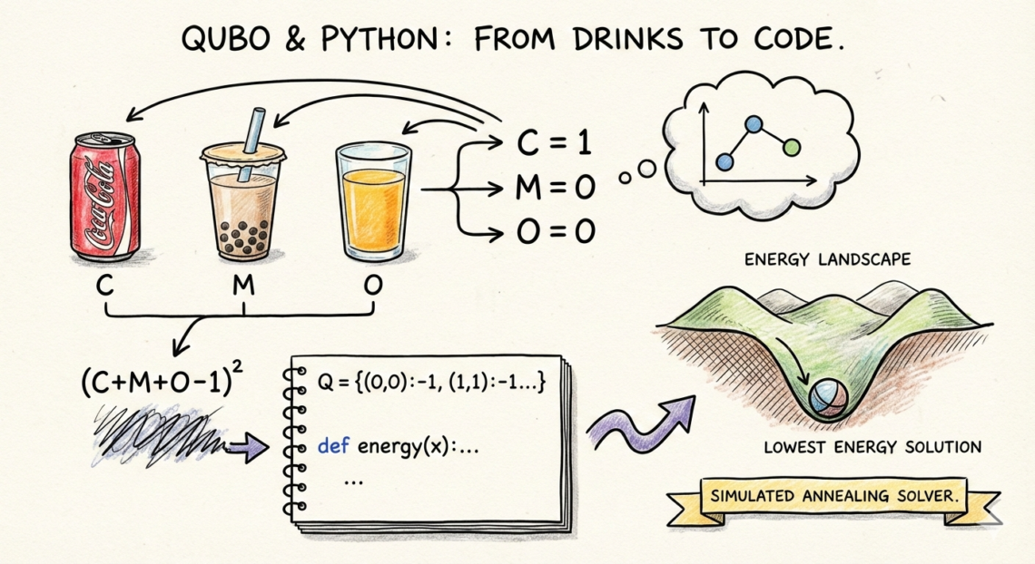
Step 4: Represent QUBO in Python

We store QUBO as a dictionary.

import itertools

# Variable order: C=0, M=1, O=2
Q = {
    (0, 0): -1,
    (1, 1): -1,
    (2, 2): -1,
    (0, 1): 2,
    (0, 2): 2,
    (1, 2): 2,
}

Each entry means:

(i, i) → node weight
(i, j) → edge penalty

Step 5: Define Energy Function

def energy(x):
    e = 0
    for (i, j), w in Q.items():
        e += w * x[i] * x[j]
    return e

This function:

Takes a solution like (1, 0, 0)
Calculates total energy

This is exactly how solvers “see” your graph.

Step 6: Brute Force Solve

Because we only have 3 variables, we can try all combinations.

best = None

for x in itertools.product([0, 1], repeat=3):
    e = energy(x)
    print(x, e)
    if best is None or e < best[1]:
        best = (x, e)
print("Best solution:", best)

You will observe:

Invalid choices → higher energy
Valid choices → lowest energy

Step 7: Interpret the Result

Valid lowest-energy solutions:

(1, 0, 0) → Coke
(0, 1, 0) → Milk Tea
(0, 0, 1) → Orange Juice

All are equally good.

Why?

Because we added rules, not preferences.

Step 8: Add Preferences (Objective)

Let’s say:

Coke is preferred
Milk Tea is disliked

Q[(0, 0)] += -2  # reward Coke
Q[(1, 1)] += 3   # penalize Milk Tea

Re-run the solver.

Now the energy landscape tilts.

One solution becomes the deepest valley.

What You Just Learned

QUBO becomes simple Python code
Solvers only compare energies
Graph intuition directly matches behavior
You don’t need special tools to start

Scaling up Step 9: Simulated Annealing (Conceptual)

Brute force helped us see everything.

But it breaks very quickly.

When variables grow:

Combinations explode
Brute force becomes impossible

This is where Simulated Annealing (SA) enters.

How Simulated Annealing Works

From Chapter 5 and the graph view:

QUBO = energy landscape
Valleys = good solutions
Hills = bad solutions

Simulated Annealing:

Starts at a random configuration
Flips one variable (node)
Measures energy change
Sometimes accepts worse moves
Gradually becomes more conservative

Early stage:

Explores widely
Jumps across hills

Late stage:

Settles into a deep valley

This is how solvers escape local minima.

Why This Matters for Real Problems

Most real QUBO problems:

Have hundreds or thousands of variables
Cannot be solved exactly
Need good solutions fast

Simulated Annealing:

Trades perfection for speed
Handles noisy, complex graphs
Works well with QUBO structure

This is why it is widely used in practice.

Step 10 — Simulated Annealing in Python (Hands-On)

Now let’s see real code.

We will use a ready-made solver, just like engineers do in real projects.

Below is an example using Fixstars Amplify (quantum-inspired, runs on classical hardware).

Install Library

pip install amplify

Define the Same QUBO Problem

from amplify import BinarySymbolGenerator, solve
from amplify.client import FixstarsClient

# Create binary variables
q = BinarySymbolGenerator()
C, M, O = q.array(3)
# Exactly-one constraint
qubo = (C + M + O - 1) ** 2
# Add preferences
qubo += -2 * C      # prefer Coke
qubo += 3 * M       # avoid Milk Tea

Run Simulated Annealing Solver

client = FixstarsClient()
client.parameters.timeout = 1000  # milliseconds

result = solve(qubo, client)
best = result.best
print("Solution:", best.values)
print("Energy:", best.energy)

Output Interpretation

Example output:

Solution: [1, 0, 0]
Energy: -2.0

Meaning:

Coke = ON
Milk Tea = OFF
Orange Juice = OFF

The solver:

Explored many configurations
Escaped local minima
Found the deepest valley

All without brute force.

What Just Happened

Under the hood, the solver:

Flipped nodes ON/OFF
Measured energy change
Sometimes accepted worse moves
Slowly settled into a low-energy state

Exactly the annealing behavior we discussed conceptually.

What You’ve Achieved So Far

You can now:

Build QUBO models
Understand them as graphs
Solve small problems exactly
Understand how solvers scale

You are no longer “reading about QUBO”.

You are using it.

What’s Next

In the next chapter, we will:

Introduce the Ising model
See how QUBO maps to Ising

This connects modeling to real solvers and machines.